What Are the Differences Between Discrete and Continuous Probability Distributions
This article was published as a part of the Data Science Blogathon.
Introduction
Today, let us talk about one of the foundational concepts of Statistics: Probability Distributions. They help understand the data better and act as a basis for understanding further statistical concepts such as Confidence Intervals and Hypothesis testing.
Informal Definition
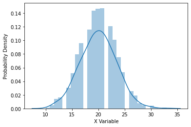
Let X be a random variable that has more than one possible outcome. Plot the probability on the y-axis and the outcome on the x-axis. If we repeat the experiment many times and plot the probability of each possible outcome, we get a plot that represents the probabilities. This plot is called the probability distribution (PD). The height of the graph for X gives the probability of that outcome.
Types of Probability Distributions
There are two types of distributions based on the type of data generated by the experiments.
1. Discrete probability distributions
These distributions model the probabilities of random variables that can have discrete values as outcomes. For example, the possible values for the random variable X that represents the number of heads that can occur when a coin is tossed twice are the set {0, 1, 2} and not any value from 0 to 2 like 0.1 or 1.6.
Examples: Bernoulli, Binomial, Negative Binomial, Hypergeometric, etc.,
2. Continuous probability distributions
These distributions model the probabilities of random variables that can have any possible outcome. For example, the possible values for the random variable X that represents weights of citizens in a town which can have any value like 34.5, 47.7, etc.,
Examples: Normal, Student's T, Chi-square, Exponential, etc.,
Terminologies
Each PD provides us extra information on the behavior of the data involved. Each PD is given by a probability function that generalizes the probabilities of the outcomes.
Using this, we can estimate the probability of a particular outcome(discrete) or the chance that it lies within a particular range of values for any given outcome(continuous). The function is called a Probability Mass function (PMF) for discrete distributions and a Probability Density function (PDF) for continuous distributions. The total value of PMF and PDF over the entire domain is always equal to one.
Cumulative Distribution Function
The PDF gives the probability of a particular outcome whereas the Cumulative Distribution Function gives the probability of seeing an outcome less than or equal to a particular value of the random variable. CDFs are used to check how the probability has added up to a certain point. For example, if P(X = 5) is the probability that the number of heads on flipping a coin is 5 then, P(X <= 5) denotes the cumulative probability of obtaining 1 to 5 heads.
Cumulative distribution functions are also used to calculate p-values as a part of performing hypothesis testing.
Discrete Probability Distributions
There are many discrete probability distributions to be used in different scenarios. We will discuss Discrete distributions in this post. Binomial and Poisson distributions are the most discussed ones in the following list.
1. Bernoulli Distribution
This distribution is generated when we perform an experiment once and it has only two possible outcomes – success and failure. The trials of this type are called Bernoulli trials, which form the basis for many distributions discussed below. Let p be the probability of success and 1 – p is the probability of failure.
The PMF is given as
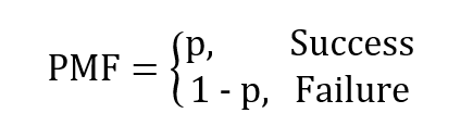
One example of this would be flipping a coin once. p is the probability of getting ahead and 1 – p is the probability of getting a tail. Please note down that success and failure are subjective and are defined by us depending on the context.
2. Binomial Distribution
This is generated for random variables with only two possible outcomes. Let p denote the probability of an event is a success which implies 1 – p is the probability of the event being a failure. Performing the experiment repeatedly and plotting the probability each time gives us the Binomial distribution.
The most common example given for Binomial distribution is that of flipping a coin n number of times and calculating the probabilities of getting a particular number of heads. More real-world examples include the number of successful sales calls for a company or whether a drug works for a disease or not.
The PMF is given as,
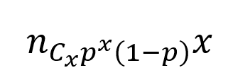
where p is the probability of success, n is the number of trials and x is the number of times we obtain a success.
3. Hypergeometric Distribution
Consider an event of drawing a red marble from a box of marbles with different colors. The event of drawing a red ball is a success and not drawing it is a failure. But each time a marble is drawn it is not returned to the box and hence this affects the probability of drawing a ball in the next trial. The hypergeometric distribution models the probability of k successes over n trials where each trial is conducted without replacement. This is unlike the binomial distribution where the probability remains constant through the trials.
The PMF is given as,
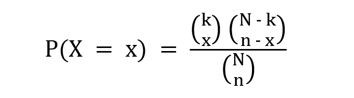
where k is the number of possible successes, x is the desired number of successes, N is the size of the population and n is the number of trials.
4.Negative Binomial Distribution
Sometimes we want to check how many Bernoulli trials we need to make in order to get a particular outcome. The desired outcome is specified in advance and we continue the experiment until it is achieved. Let us consider the example of rolling a dice. Our desired outcome, defined as a success, is rolling a 4. We want to know the probability of getting this outcome thrice. This is interpreted as the number of failures (other numbers apart from 4) that will occur before we see the third success.
The PMF is given as,
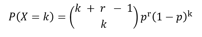
where p is the probability of success, k is the number of failures observed and r is the desired number of successes until the experiment is stopped.
Like in Binomial distribution, the probability through the trials remains constant and each trial is independent of the other.
5. Geometric Distribution
This is a special case of the negative binomial distribution where the desired number of successes is 1. It measures the number of failures we get before one success. Using the same example given in the previous section, we would like to know the number of failures we see before we get the first 4 on rolling the dice.
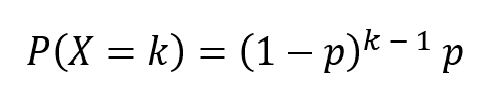
where p is the probability of success and k is the number of failures. Here, r = 1.
6. Poisson Distribution
This distribution describes the events that occur in a fixed interval of time or space. An example might make this clear. Consider the case of the number of calls received by a customer care center per hour. We can estimate the average number of calls per hour but we cannot determine the exact number and the exact time at which there is a call. Each occurrence of an event is independent of the other occurrences.
The PMF is given as,
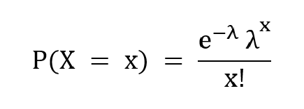
where λ is the average number of times the event has occurred in a certain period of time, x is the desired outcome and e is the Euler's number.
7. Multinomial Distribution
In the above distributions, there are only two possible outcomes – success and failure. The multinomial distribution, however, describes the random variables with many possible outcomes. This is also sometimes referred to as categorical distribution as each possible outcome is treated as a separate category. Consider the scenario of playing a game n number of times. Multinomial distribution helps us to determine the combined probability that player 1 will win x1times, player 2 will win x2times and player k winsx ktimes.
The PMF is given as,
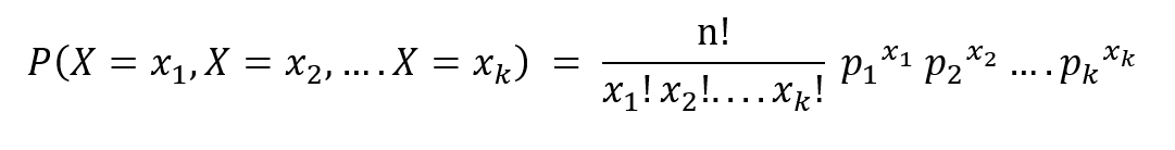
where n is the number of trials, p1,……pk denote the probabilities of the outcomes x1……xk respectively.
In this post, we have defined probability distributions and briefly discussed different discrete probability distributions. Let me know your thoughts on the article in the comments section below.
References
1. https://www.statisticshowto.com/
2. https://stattrek.com/
3. Wikipedia
About Me
I am a former software engineer, working on transitioning into Data Science. I am a master's student in Data Science. Please feel free to connect with me on https://www.linkedin.com/in/priyanka-madiraju/
The media shown in this article are not owned by Analytics Vidhya and is used at the Author's discretion.
foglemannorgarehe.blogspot.com
Source: https://www.analyticsvidhya.com/blog/2021/01/discrete-probability-distributions/
0 Response to "What Are the Differences Between Discrete and Continuous Probability Distributions"
Postar um comentário